draw line between two vectors matlab 3d
What is Matlab?
MATLAB is a linguistic communication used for technical computing. As most of us will agree, an easy to use surround is a must for integrating tasks of computing, visualizing and finally programming. MATLAB does the aforementioned by providing an environs that is non only easy to utilize but also, the solutions that nosotros get are displayed in terms of mathematical notations which most of us are familiar with.
Uses of MATLAB for Calculating
MATLAB is used in many unlike ways, following are the list where it is commonly used.
- Ciphering
- Development of Algorithms
- Modeling
- Simulation
- Prototyping
- Data analytics (Analysis and Visualization of data)
- Applied science & Scientific graphics
- Awarding development
MATLAB provides its user with a handbasket of functions and tools, in this article we will understand About 3-dimensional plots in MATLAB.
- Plots are created for data visualization.
- Information visualization is very powerful in getting the look and feel of the data in simply one glance.
- Data plots take a number of uses from comparing sets of data to tracking information changes over time.
Plots tin exist created using graphic functions or interactively using the MATLAB Desktop.
Types of 3D Plots in MATLAB
Below we take discussed the types of 3D plots in MATLAB used in computing.
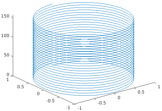
1. PLOT3 (Line Plots)
Plot3 helps in creating 3D lines or Point Plots.
Plot3(10,y,z): If x,y,z are vectors of the same length, and then this function will create a set up of coordinates connected by line segments. If we specify at least one of x, y or z as vectors, information technology will plot multiple sets of coordinates for the same prepare of axes.
Code:
A= 0: pi/100; 50*pi;
                sa= sin(a);
                ca=cos(a);
                plot3(sa, ca, a)
Output:
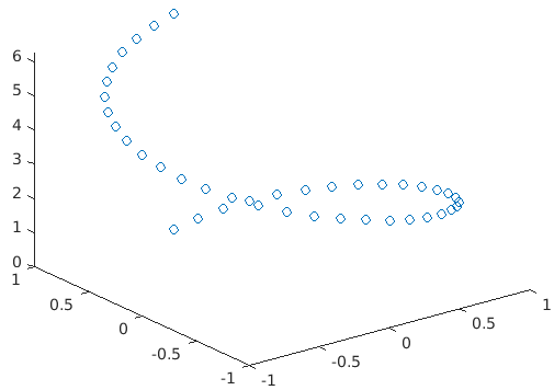
plot3( X , Y , Z , LineSpec): This function will create the plot using the specified line mode, mark, and color.
Code:
A= 0:pi/twenty:2*pi;
                sa= sin(a);
                ca=cos(a) ;
                plot3(sa, ca, a, 'o')
Output:
plot3(X1, Y1, Z1,…, Xn, Yn, Zn): This function volition plot multiple coordinates for the same set of axes.
Code:
a= 0:pi/100*pi;
                xa1= sin(a).cos(ten*a);
                ya1=sin(a).*sin(x*a) ;
                za1=cos(a);
                xa2= sin(a).cos(15*a);
                ya2=sin(a).*sin(15*a) ;
                za2=cos(a);
                Plot3(xa1,ya1,za1,xa2,ya2,za2)
Output:
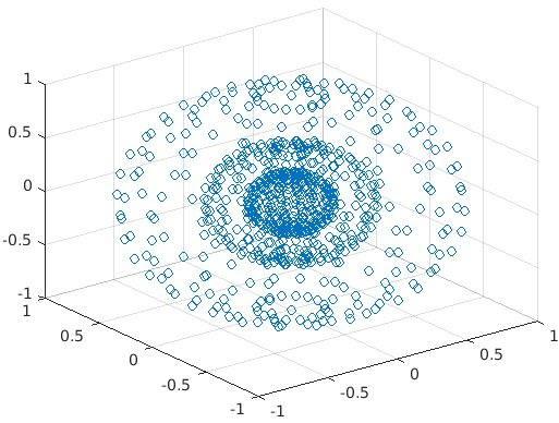
2. SCATTER3 (3D scatter Plot)
scatter3( 10 , Y , Z ): This function will create circles at the vector locations of x, y, and z.
Case:
X, y, z are vector spheres.
Code:
[10,Y,Z] = SPHERE(ten)
                ten = [0.5*X(:); 0.25*X(:); X(:)];
                y = [0.5*Y(:); 0.25*Y(:); Y(:)];
                z = [0.5*Z(:); 0.25*Z(:); Z(:)];
Output:
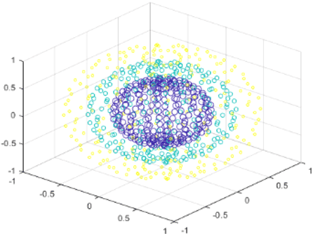
scatter3( X , Y , Z , A , C): This part will create a plot with a circle that volition have size A from the argument. If A is scalar, the size of the circles volition exist equal. For the specific size of the circle, we will have to define A as a vector.
Code:
[X, Y, Z] = sphere(20);
                x = [0.5*X(:); 0.75*Ten(:); Ten(:)];
                y = [0.5*Y(:); 0.75*Y(:); Y(:)];
                z = [0.5*Z(:); 0.75*Z(:); Z(:)];
                scatter3(x, y, z)
Define a vector to specify the marker sizes.
a = repmat([fifty,ten,2],numel(Ten),one);
                C = repmat([1,2,3],numel(X),ane);
                a = a(:);
                c = c(:);
Output:
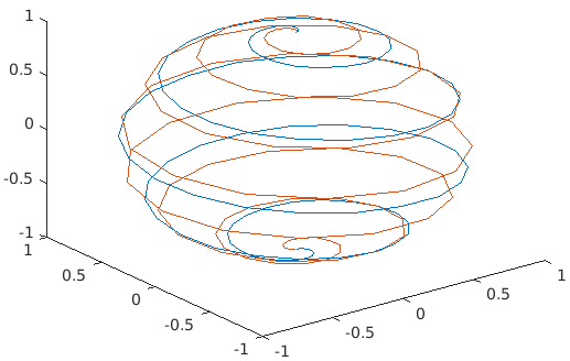
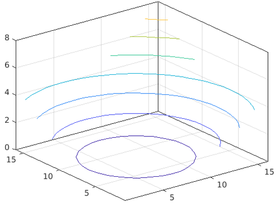
iii. CONTOUR3 (3D contour plots)
contour3(Z): Z is a matrix and this function will create a 3-D contour plot which will have the isolines of matrix z will have the tiptop details of x and y plane. The ten & y coordinates in the airplane are column and row indices of Z. Contour lines are selected by MATLAB automatically.
Code:
[X,Y] = meshgrid(-1:0.20:2);
                Z = X.^2 + Y.^two;
                contour3(Z)
Output:
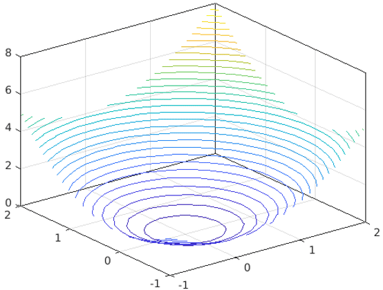
Define contour levels equally 30, and display the results within x and y limits.
Code:
Contour3(X,Y,Z,30)
Output:
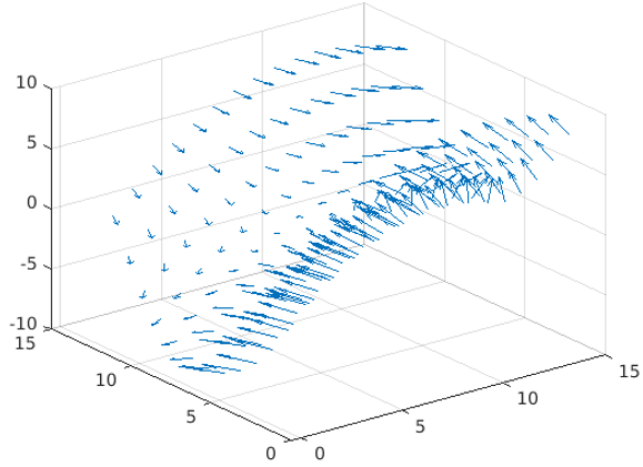
iv. QUIVER3 (Velocity Plot)
3D quiver plot creates vectors with components (u,v,due west) at the points (x,y,z), where u, v, w, x, y, and z are real values.
Code:
ten = -3:0.5:three;
                y = -iii:0.5:iii;
                [X,Y] = meshgrid(x, y);
                Z = Y.^2 - X.^ii;
                [U,V,Due west] = surfnorm(Z);
Output:
5. FILL3 (3D filled polygon plot)
This function helps in creating apartment shaped and Gouraud polygons (to get different shades of light).
fill3(X, Y, Z, C): It helps in creating filled polygons with vertices x, y, z. The x, y, z values tin be number, duration, and DateTime, etc.
Code:
Ten = [1 2 iii 4; 1 1 3 two; 0 ane 2 1];
                Y = [2 2 ane one; 1 ii 1 ii; 1 i 0 0];
                Z = [1 i i ane; 1 0 one 0; 0 0 0 0];
                C = [0.5000 1.0000 1.0000 0.5000;
                1.0000 0.5000 0.5000 0.1667;
                0.3330 0.3330 0.5000 0.5000];
Output:
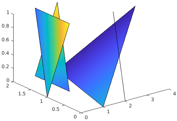
In the in a higher place figure, we can clearly see the Gouraud effect.
Conclusion – 3D Plots in Matlab
Data visualization becomes a very powerful technique when nosotros have to understand how our information is behaving. It also tells us visually, how a particular function is changing when it is supplied with different values. iii D plot in MATLAB is a tool which is very helpful in visualizing the beliefs of data.
Recommended Articles
This is a guide to 3D Plots in Matlab. Here we discuss what is Matlab, uses Matlab and types of 3D plot in Matlab for calculating. You tin also go through our other related articles to acquire more –
- What are the MATLAB Functions?
- Bessel Functions in MATLAB
- Advantages of Matlab for Programming
- R Data Types and Structures
- Steps and Methods to Utilize Matlab Comet()
- How to Use Matlab?
- Acquire the Examples of Contour plot in Matlab
- Examples of Meshgrid in Matlab
Source: https://www.educba.com/3d-plots-in-matlab/
0 Response to "draw line between two vectors matlab 3d"
Post a Comment